Where Can I Lookup A Federally Registered Business

Tip:Try using the new XLOOKUP function, an improved version of VLOOKUP that works in whatever direction and returns verbal matches by default, making it easier and more convenient to apply than its predecessor.

Utilize VLOOKUP when you lot need to detect things in a table or a range by row. For case, look up a cost of an automotive office past the part number, or find an employee name based on their employee ID.

In its simplest course, the VLOOKUP office says:

=VLOOKUP(What you want to look upwardly, where you want to wait for information technology, the column number in the range containing the value to render, return an Guess or Exact friction match – indicated as i/True, or 0/Faux).

Tip:The secret to VLOOKUP is to organize your data then that the value you lot look upwardly (Fruit) is to the left of the render value (Amount) y'all want to find.

Utilize the VLOOKUP function to look up a value in a table.

Syntax

VLOOKUP (lookup_value, table_array, col_index_num, [range_lookup])

For instance:

• =VLOOKUP(A2,A10:C20,2,Truthful)

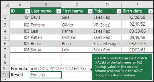
• =VLOOKUP("Fontana",B2:E7,2,FALSE)

• =VLOOKUP(A2,'Client Details'!A:F,3,FALSE)

Argument proper noun	Description
lookup_value    (required)	The value you want to expect upwardly. The value yous desire to look upwardly must be in the first column of the range of cells you specify in the table_array statement. For instance, if table-array spans cells B2:D7, then your lookup_value must be in column B. Lookup_value tin be a value or a reference to a cell.
table_array    (required)	The range of cells in which the VLOOKUP will search for the lookup_value and the render value. You can utilise a named range or a tabular array, and you can utilise names in the statement instead of cell references. The commencement column in the prison cell range must contain the lookup_value . The cell range likewise needs to include the return value you desire to find. Learn how to select ranges in a worksheet.
col_index_num    (required)	The column number (starting with 1 for the left-most cavalcade of table_array ) that contains the return value.
range_lookup   (optional)	A logical value that specifies whether yous want VLOOKUP to detect an estimate or an exact lucifer: Judge friction match - 1/Truthful assumes the starting time cavalcade in the table is sorted either numerically or alphabetically, and will so search for the closest value. This is the default method if you don't specify one. For example, =VLOOKUP(90,A1:B100,2,True). Exact match - 0/Imitation searches for the exact value in the kickoff column. For example, =VLOOKUP("Smith",A1:B100,ii,FALSE).

How to get started

At that place are 4 pieces of information that yous volition need in order to build the VLOOKUP syntax:

1. The value yous desire to look up, also chosen the lookup value.

2. The range where the lookup value is located. Call up that the lookup value should e'er be in the first column in the range for VLOOKUP to work correctly. For case, if your lookup value is in jail cell C2 then your range should commencement with C.

3. The column number in the range that contains the return value. For example, if you specify B2:D11 as the range, y'all should count B equally the first cavalcade, C as the second, then on.

4. Optionally, you can specify TRUE if you want an approximate lucifer or FALSE if you lot want an exact match of the return value. If you don't specify anything, the default value will e'er be TRUE or gauge match.

Now put all of the above together as follows:

=VLOOKUP(lookup value, range containing the lookup value, the cavalcade number in the range containing the return value, Gauge friction match (TRUE) or Exact friction match (FALSE)).

Examples

Here are a few examples of VLOOKUP:

Example i

Instance 2

Example iii

Instance 4

Example v

You can utilise VLOOKUP to combine multiple tables into one, as long equally one of the tables has fields in common with all the others. This tin can be peculiarly useful if you need to share a workbook with people who have older versions of Excel that don't support data features with multiple tables every bit information sources - by combining the sources into i table and changing the data feature's data source to the new table, the data feature tin can be used in older Excel versions (provided the information feature itself is supported by the older version).

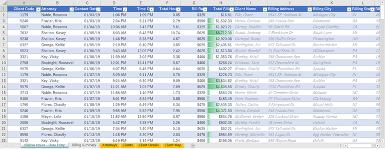Here, columns A-F and H have values or formulas that only use values on the worksheet, and the rest of the columns use VLOOKUP and the values of cavalcade A (Client Lawmaking) and column B (Attorney) to get information from other tables.

1. Re-create the table that has the common fields onto a new worksheet, and give it a proper noun.

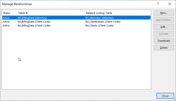
2. Click Data > Information Tools > Relationships to open the Manage Relationships dialog box.

   

3. For each listed relationship, note the post-obit:

   • The field that links the tables (listed in parentheses in the dialog box). This is the lookup_value for your VLOOKUP formula.

   • The Related Lookup Table name. This is the table_array in your VLOOKUP formula.

   • The field (column) in the Related Lookup Table that has the data you want in your new column. This information is not shown in the Manage Relationships dialog - yous'll have to wait at the Related Lookup Table to see which field yous want to recollect. You desire to annotation the column number (A=ane) - this is the col_index_num in your formula.

4. To add a field to the new table, enter your VLOOKUP formula in the outset empty cavalcade using the data yous gathered in step 3.

   In our case, cavalcade G uses Attorney (the lookup_value ) to get the Beak Charge per unit data from the fourth column ( col_index_num = 4) from the Attorneys worksheet table, tblAttorneys (the table_array ), with the formula =VLOOKUP([@Attorney],tbl_Attorneys,four,False).

   The formula could likewise utilize a cell reference and a range reference. In our case, it would exist =VLOOKUP(A2,'Attorneys'!A:D,4,False).

5. Continue adding fields until you accept all the fields that you lot demand. If y'all are trying to prepare a workbook containing information features that use multiple tables, change the data source of the data feature to the new table.

Problem	What went incorrect
Wrong value returned	If range_lookup is True or left out, the offset column needs to exist sorted alphabetically or numerically. If the kickoff column isn't sorted, the return value might be something you don't expect. Either sort the starting time column, or apply False for an exact match.
#Due north/A in prison cell	If range_lookup is TRUE, then if the value in the lookup_value is smaller than the smallest value in the commencement cavalcade of the table_array , you'll become the #Due north/A error value. If range_lookup is False, the #Due north/A error value indicates that the exact number isn't found. For more data on resolving #N/A errors in VLOOKUP, see How to right a #N/A error in the VLOOKUP function.
#REF! in cell	If col_index_num is greater than the number of columns in tabular array-array , y'all'll get the #REF! error value. For more than information on resolving #REF! errors in VLOOKUP, run across How to correct a #REF! fault.
#VALUE! in cell	If the table_array is less than 1, you'll get the #VALUE! mistake value. For more data on resolving #VALUE! errors in VLOOKUP, see How to correct a #VALUE! error in the VLOOKUP part.
#NAME? in cell	The #Name? error value usually means that the formula is missing quotes. To wait upward a person's proper noun, make sure you utilise quotes around the name in the formula. For example, enter the proper name as "Fontana" in =VLOOKUP("Fontana",B2:E7,2,FALSE). For more data, see How to correct a #Proper name! error.
#SPILL! in cell	This particular #SPILL! error usually means that your formula is relying on implicit intersection for the lookup value, and using an entire cavalcade as a reference. For instance, =VLOOKUP(A:A,A:C,ii,FALSE). You lot tin can resolve the issue past anchoring the lookup reference with the @ operator like this: =VLOOKUP(@A:A,A:C,two,Fake). Alternatively, you can use the traditional VLOOKUP method and refer to a single cell instead of an entire column: =VLOOKUP(A2,A:C,ii,False).

Do this	Why
Utilize accented references for range_lookup	Using absolute references allows you to make full-downwardly a formula so that it always looks at the same exact lookup range. Learn how to apply absolute prison cell references.
Don't store number or date values equally text.	When searching number or date values, be certain the information in the first cavalcade of table_array isn't stored as text values. Otherwise, VLOOKUP might return an incorrect or unexpected value.
Sort the first column	Sort the first column of the table_array before using VLOOKUP when range_lookup is TRUE.
Use wildcard characters	If range_lookup is Fake and lookup_value is text, yous tin can utilize the wildcard characters—the question mark (?) and asterisk (*)—in lookup_value . A question marker matches any single grapheme. An asterisk matches any sequence of characters. If you lot desire to discover an actual question marker or asterisk, type a tilde (~) in front end of the character. For example, =VLOOKUP("Fontan?",B2:E7,2,Fake) will search for all instances of Fontana with a concluding letter that could vary.
Make sure your data doesn't contain erroneous characters.	When searching text values in the first cavalcade, make sure the information in the first cavalcade doesn't have leading spaces, trailing spaces, inconsistent use of straight ( ' or " ) and curly ( ' or ") quotation marks, or nonprinting characters. In these cases, VLOOKUP might render an unexpected value. To go accurate results, effort using the CLEAN function or the TRIM part to remove trailing spaces later tabular array values in a prison cell.

Need more than help?

You can always ask an skilful in the Excel Tech Customs or become back up in the Answers customs.

Meet As well

Quick Reference Card: VLOOKUP refresher
Quick Reference Carte: VLOOKUP troubleshooting tips
How to correct a #VALUE! error in the VLOOKUP function
How to correct a #Northward/A fault in the VLOOKUP role
Overview of formulas in Excel
How to avoid cleaved formulas
Detect errors in formulas
Excel functions (alphabetical)
Excel functions (by category)
VLOOKUP (free preview)

Source: https://support.microsoft.com/en-us/office/vlookup-function-0bbc8083-26fe-4963-8ab8-93a18ad188a1

Posted by: mullanaforeg.blogspot.com

Share this post